Geometry Optimization
This is the first step before anything is done. To get accurate calculations on anything, you have to first optimize the structure to its lowest energy (and therefore most stable) structure. You can read more about optimization methods here. There's also some nice video lectures by Dr. David Sherrill here and by Dr. Chris Cramer here. General information for Gaussian setups can be found here.
Firstly, you want to begin with building your structure. I found it easiest to build it on ChemDraw to make sure it looks good in regards to visualizing the number of hydrogens, single/double/triple bonds, etc. From there I would export it as SMILES. You can export it as an inchi key as well.
I would then import it into a visualizer like WebMO to get the coordinates. If it was a small structure that would compute in less than an hour, I'd just do it there. Otherwise, for most of my structures I'd use a cluster like Clemson University's Palmetto Cluster and take advantage of the available number of CPUs to speed up the process.
Firstly, you have to setup the batch file in order to allocate proper resources, among other things. Each cluster has their own documentation. Palmetto's is here. If I remember correctly, the documentation was on Github when I first started out but I might be wrong. I feel like it wasn't this well documented a year ago. Keep in mind I used the template below a year ago as well, so node names might have changed. Anyways, I used a setup like this which pretty much hits everything someone might need:
#PBS -N g16
#PBS -q skystd
#PBS -1 select=1:ncpus=20:men=40gb,walltime=3:00:00
#PBS -M [email]
#PBS -m abe

input=[name].inp

module load gaussian/g16-sky-avx2

filename='basename $input .inp'
cd $PBS_0_WORKDIR

export GAUSS_LFLAGS='-opt "Isnet.Node.lindarsharg: ssh"'

nodes='cat $PBS_NODEFILE | uniq'
scratch="/local_scratch/pbs.$PBS_JOBID"

pbsdsh sleep 10

export GAUSS_SCRDIR=$scratch

tmpinput=${filename}_tmp.inp
nodelist='cat $PBS_NODEFILE | uniq | tr '\n' "," | sed 's|,$||''
echo "%NProcShared=" $0MP_NUM_THREADS > $tmpinput
echo "%LindaWorkers=" $nodelist >> $tmpinput
cat $input >> $tmpinput

g16 $tmpinput

rm $tmpinput
mv ${filename}_tmp.log ${filename}.log
For the actual input file of the molecule, it's important to keep the following in mind:
- Each job specification is different, a geometry optimization input is going to be different from a molecular orbital input and so on.
- Keep the output coordinates of the geometry optimization. They will be used as the input for any further calculations, for the reasons we mentioned above.
- You're also gonna want to keep the method/basis set consistent for the same reasons.
- Picking a method/basis set is dependent on literature in your field. In my case, I looked into literature of benchmark calculations comparing different methods and basis sets for organic semiconducting molecules. Lots of publications are pretty good on citing them as well, so you'll be put on a good path. I'll elaborate on this shortly.
Let's say you were working with a huge molecule, namely this one:
Here's what the molecule input file would look like:
 %mem=30gb
 %chk=P2n2ccH
 #n B3LYP/6-31G** OPT FREQ

P2n2 all c H

 0 1
 C                     0.        0.        0.
 C                     0.08884  -1.37552  -0.19286
 C                     1.32481  -2.00298  -0.43676
 C                     2.51732  -1.28067  -0.49434
 C                     2.41651   0.09367  -0.29706
 C                     1.18344   0.74394  -0.05581
 N                     1.36534   2.11419   0.08859
 C                     2.65535   2.30481  -0.03338
 N                     3.36938   1.1191   -0.24832
 C                     4.74247   1.04032  -0.53271
 C                     5.50961   2.29316  -0.2069
 C                     4.78382   3.53718  -0.1382
 C                     3.37193   3.56026  -0.03697
 C                     2.6866    4.77932   0.06445
 C                     3.37707   5.98028   0.04261
 C                     4.78094   6.00916  -0.05659
 C                     5.49271   4.77275  -0.1202
 C                     6.91141   4.77276  -0.19428
 C                     7.62032   3.53719  -0.17625
 C                     9.0322    3.56027  -0.27754
 C                     9.74879   2.30481  -0.28114
 N                     9.03475   1.11908  -0.06638
 C                     7.66173   1.0404    0.21846
 C                     6.89453   2.29318  -0.10747
 O                     7.19379   0.05592   0.75239
 C                     9.98763   0.09367  -0.01754
 C                     11.22072   0.74397  -0.25861
 N                     11.03881   2.11422  -0.40295
 C                     12.40417   0.00004  -0.31434
 C                     12.31532  -1.3755   -0.1216
 C                     11.07934  -2.00299   0.12211
 C                     9.88681  -1.28069   0.1796
 H                     8.93318  -1.75212   0.37712
 N                     11.1225  -3.03438   0.30358
 C                     12.33518  -3.52883   0.28837
 N                     13.32073  -2.56309   0.04758
 C                     14.70597  -2.78928   0.09658
 C                     15.09304  -4.24224   0.03866
 C                     14.11443  -5.22367   0.4364
 C                     12.74318  -4.89066   0.55034
 C                     11.80167  -5.86764   0.90409
 C                     12.2006   -7.16723   1.17139
 C                     13.55239  -7.54701   1.07165
 C                     14.5149   -6.57015   0.6733
 C                     15.88184  -6.93311   0.53933
 C                     16.82416  -5.97607   0.06435
 C                     18.1853   -6.3521   -0.03624
 C                     19.14389  -5.37334  -0.49758
 N                     18.67837  -4.12846  -0.93975
 C                     17.32763  -3.75562  -1.03455
 C                     16.39111  -4.63827  -0.25472
 O                     16.98489  -2.84193  -1.75631
 C                     19.80048  -3.44033  -1.41846
 C                     20.88335  -4.31907  -1.18031
 N                     20.44015  -5.51249  -0.62276
 C                     22.18546  -3.92985  -1.51211
 C                     22.3617   -2.67057  -2.07805
 C                     21.27052  -1.81294  -2.31172
 C                     19.96413  -2.18     -1.98651
 H                     19.11743  -1.53245  -2.17211
 H                     21.4508   -0.83538  -2.75891
 H                     23.36579  -2.34169  -2.3459
 H                     23.01961  -4.5987   -1.32949
 C                     18.5922   -7.64785   0.31238
 C                     17.66658  -8.58724   0.737
 C                     16.30213  -8.2613    0.85335
 C                     15.31746  -9.21578   1.2688
 C                     13.99969  -8.87694   1.36217
 H                     13.26278  -9.61386   1.66836
 H                     15.64356  -10.22522  1.50231
 H                     17.99187  -9.59336   0.98541
 H                     19.64525  -7.89346   0.23211
 H                     11.46391  -7.91003  1.46348
 H                     10.75962  -5.57526  0.96997
 O                     15.4805   -1.86758  0.25092
 H                     13.40207  0.55395  -0.35778
 C                     9.71752   4.77933  -0.37899
 C                     9.02705   5.98029  -0.35715
 C                     7.62319   6.00916  -0.25792
 C                     6.88184   7.23448  -0.21125
 C                     5.52228   7.23448  -0.10328
 H                     4.97422   8.1712   -0.05839
 H                     7.42989   8.17121  -0.25616
 H                     9.57129   6.91838  -0.4168
 H                     10.79803  4.75425  -0.46602
 H                     2.83282   6.91837   0.10224
 H                     1.6061    4.75424   0.15144
 O                     5.2105    0.05576  -1.06642
 H                     3.47094  -1.75207  -0.69197
 H                     1.35301  -3.07762  -0.58812
 H                    -0.81273  -1.97941  -0.15758
 H                    -0.94781   0.49315   0.187
 ***put a blank line at the end here***
So what does this entail?
- Line 1: instructs Gaussian to have a maximum storage of 30 gigabytes
- Line 2: instructs Gaussian to keep a checkpoint of the following name
- Line 3: provides the Gaussian route, i.e. the instruction specifying the calculation(s) to be performed. B3LYP/6-31G(d,p) indicates the type of calculation (DFT hybrid functional B3LYP) and the basis set (6-31G(d,p)) to be used. Opt specifies a geometry optimization calculation.
- Line 5: contains the calculation title.
- Line 7: specifies charge and multiplicity.
- Lines 8-99: starting-point geometry, in XYZ format. Each line corresponds to a new atom, indicating atom type and coordinates.
- Line 100: keep blank, otherwise the calculation won't happen.
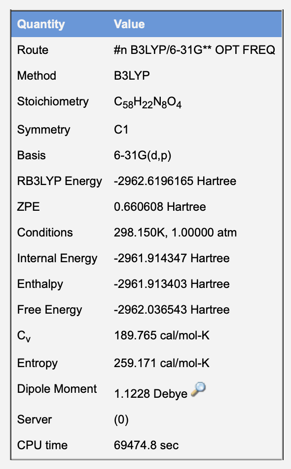
Zero-point correction=                               0.660608 (Hartree/Particle)
Thermal correction to Energy=                  	     0.705269
Thermal correction to Enthalpy=                      0.706214
Thermal correction to Gibbs Free Energy=             0.583073
Sum of electronic and zero-point Energies=          -2961.959009
Sum of electronic and thermal Energies=             -2961.914347
Sum of electronic and thermal Enthalpies=           -2961.913403
Sum of electronic and thermal Free Energies=        -2962.036543
You can avoid sorting through the mess of the output file by having access to graphical interface softwares like GaussView, WebMo or the free counterpart, Avogadro. Usually, you'll have access without having to pay through your educational institution. All that entails is saving the output file the Gaussian calculation and importing it into the respective software. WebMo has some pretty good documentation so it's easy to follow. Once you import it, all the necessary output data is organized into nice tables, like the one you see below.